
K-means Clustering Algorithm for Social Good!
When we have all data online it will be great for humanity. It is a prerequisite to solving many problems that humankind faces. - Robert Cailliau
As I mentioned in my previous posts, I would like to learn how data science algorithms and methods can be used for social good and improve human’s lives; hence, in this post, I discuss clustering method and its application in society.
As part of my M.Sc. in Management Engineering from the University of Waterloo, I wrote a thesis on “Detecting Weak Signals by Internet-Based Environmental Scanning.” This was an opportunity to apply data mining, computer tools and human judgement to predict the market potential of a new product called Micro-tile as displayed below.
 source:https://www.christiedigital.com/en-us/microtiles
I used both programming and human analysis to retrieve 40,000 HTML pages, analyze the data, and produce information that was relevant for the strategic marketing department of Christie Digital.
To succeed in my thesis, it was essential to cluster pages according to their content. I chose k-means algorithm (with each cluster accounting for no more than 10% of the overall count) and CLUTO for the clustering function. This enabled me to produce clusters with similar content (matching key words), which were ready for human analysis. I think this method is really useful in text mining and web mining area, that’s why in this post I intend to talk about k-means clustering.
Clustering
Clustering algorithm is one of the most influential and fastest method in machine learning. It is used to group large amounts of data into a number of clusters. Clustering is part of the unsupervised method which means that no training set is required. In this post, I would specifically want to discuss the K Means clustering algorithm and provide an example to undrestand how it works in R .
K Means Algorithm
Below are the steps to perform K-means algorithm:
1- Select K as the initial number of clusters.
2- Data set should be separated into k clusters randomly.
3- Compute distances between each of cluster means and all other points.
4- Assign all points to the closest centroid and move data points if they are not close to their own clusters.
5- Recompute the centroid of each cluster.
6- Repeat steps 3 and 4 until the K clusters are reached and when the assignment of the data points to cluster no longer changes.
To learn more about k-means look at this video.
Kmeans() function in R
I want to show a quick demo of applying this method in R. R has a function called k-means that can be used for k clustering.
I would like to use Lawyers’ ratings of state judges in the US Superior Court to analyze kmeans clustering. To find out more about the variables in this dataset, take a look at this link.
First, we should load all required libraries.
# load necessary libraries
library(tidyverse)
## Loading tidyverse: ggplot2
## Loading tidyverse: tibble
## Loading tidyverse: tidyr
## Loading tidyverse: readr
## Loading tidyverse: purrr
## Loading tidyverse: dplyr

## Conflicts with tidy packages ----------------------------------------------

## filter(): dplyr, stats
## lag():    dplyr, stats
# reading csv file
USJudgeRatings <- read.csv("USJudgeRatings.csv")
For kmeans() clustering to work in R, we need to ensure that all NAs are removed in the dataset.
# removing N/A
US_Judge <- na.omit(USJudgeRatings)

# use str function to see the structure of the data
str(US_Judge)
## 'data.frame':    43 obs. of  13 variables:
##  $ Judge: Factor w/ 43 levels "AARONSON,L.H.",..: 1 2 3 4 5 6 7 8 9 10 ...
##  $ CONT : num  5.7 6.8 7.2 6.8 7.3 6.2 10.6 7 7.3 8.2 ...
##  $ INTG : num  7.9 8.9 8.1 8.8 6.4 8.8 9 5.9 8.9 7.9 ...
##  $ DMNR : num  7.7 8.8 7.8 8.5 4.3 8.7 8.9 4.9 8.9 6.7 ...
##  $ DILG : num  7.3 8.5 7.8 8.8 6.5 8.5 8.7 5.1 8.7 8.1 ...
##  $ CFMG : num  7.1 7.8 7.5 8.3 6 7.9 8.5 5.4 8.6 7.9 ...
##  $ DECI : num  7.4 8.1 7.6 8.5 6.2 8 8.5 5.9 8.5 8 ...
##  $ PREP : num  7.1 8 7.5 8.7 5.7 8.1 8.5 4.8 8.4 7.9 ...
##  $ FAMI : num  7.1 8 7.5 8.7 5.7 8 8.5 5.1 8.4 8.1 ...
##  $ ORAL : num  7.1 7.8 7.3 8.4 5.1 8 8.6 4.7 8.4 7.7 ...
##  $ WRIT : num  7 7.9 7.4 8.5 5.3 8 8.4 4.9 8.5 7.8 ...
##  $ PHYS : num  8.3 8.5 7.9 8.8 5.5 8.6 9.1 6.8 8.8 8.5 ...
##  $ RTEN : num  7.8 8.7 7.8 8.7 4.8 8.6 9 5 8.8 7.9 ...
US_Judge_df <- data.matrix (US_Judge)
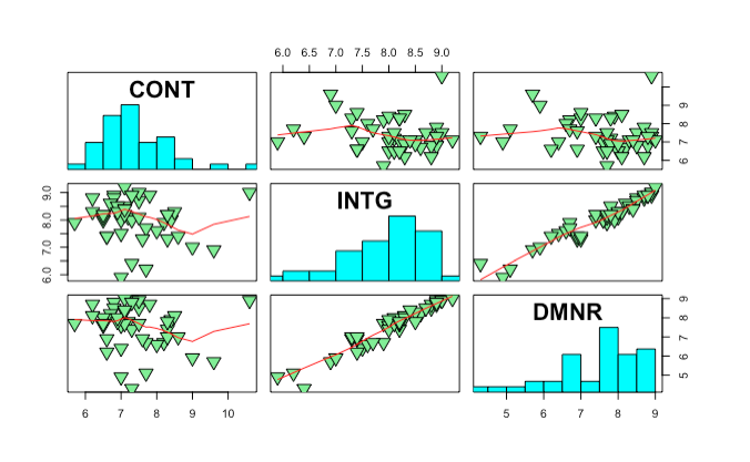
I used pairs function to display the scatter plots for the first three variables in the dataset. To learn more about pairs function, you can read further by looking at the reference I used to create these plots.
panel.hist <- function(x, ...)
{
    usr <- par("usr"); on.exit(par(usr))
    par(usr = c(usr[1:2], 0, 1.5) )
    h <- hist(x, plot = FALSE)
    breaks <- h$breaks; nB <- length(breaks)
    y <- h$counts; y <- y/max(y)
    rect(breaks[-nB], 0, breaks[-1], y, col = "cyan", ...)
}


pairs(USJudgeRatings[2:4], panel = panel.smooth,
      cex = 2, pch = 25, bg = "light green",
      diag.panel = panel.hist, cex.labels = 2, font.labels = 2)
Now we assume, the number of clusters can be 4. As mentioned above, the number of clusters will be chosen randomly, I use Kmeans() function in R. I put nstart as 30 here, it has been mentioned that nstart parameter can be any number between 20 and 50 which means that R will “try 30 different random starting assignments and then select the one with the lowest within cluster variation”. source
# using kmeans clustering algorithm
cluster_4 <- kmeans(US_Judge_df, 4, nstart = 20)

# print cluster
cluster_4
## K-means clustering with 4 clusters of sizes 9, 12, 11, 11
##
## Cluster means:
##   Judge     CONT     INTG     DMNR     DILG     CFMG     DECI     PREP
## 1  39.0 7.877778 7.700000 7.222222 7.455556 7.433333 7.522222 7.322222
## 2  17.5 7.408333 7.791667 7.066667 7.141667 6.900000 6.950000 6.875000
## 3  29.0 7.263636 8.500000 8.236364 8.418182 8.145455 8.181818 8.263636
## 4   6.0 7.281818 8.054545 7.527273 7.763636 7.481818 7.654545 7.436364
##       FAMI     ORAL     WRIT     PHYS     RTEN
## 1 7.300000 7.100000 7.211111 7.855556 7.322222
## 2 6.900000 6.708333 6.833333 7.283333 7.016667
## 3 8.290909 8.090909 8.154545 8.536364 8.363636
## 4 7.481818 7.290909 7.354545 8.109091 7.709091
##
## Clustering vector:
##  1  2  3  4  5  6  7  8  9 10 11 12 13 14 15 16 17 18 19 20 21 22 23 24 25
##  4  4  4  4  4  4  4  4  4  4  4  2  2  2  2  2  2  2  2  2  2  2  2  3  3
## 26 27 28 29 30 31 32 33 34 35 36 37 38 39 40 41 42 43
##  3  3  3  3  3  3  3  3  3  1  1  1  1  1  1  1  1  1
##
## Within cluster sum of squares by cluster:
## [1] 128.8111 211.9358 141.9927 286.4309
##  (between_SS / total_SS =  89.1 %)
##
## Available components:
##
## [1] "cluster"      "centers"      "totss"        "withinss"
## [5] "tot.withinss" "betweenss"    "size"         "iter"
## [9] "ifault"
We can see the structure of the clusters by using the following function.
# structre of the clusters
str(cluster_4)
## List of 9
##  $ cluster     : Named int [1:43] 4 4 4 4 4 4 4 4 4 4 ...
##   ..- attr(*, "names")= chr [1:43] "1" "2" "3" "4" ...
##  $ centers     : num [1:4, 1:13] 39 17.5 29 6 7.88 ...
##   ..- attr(*, "dimnames")=List of 2
##   .. ..$ : chr [1:4] "1" "2" "3" "4"
##   .. ..$ : chr [1:13] "Judge" "CONT" "INTG" "DMNR" ...
##  $ totss       : num 7077
##  $ withinss    : num [1:4] 129 212 142 286
##  $ tot.withinss: num 769
##  $ betweenss   : num 6308
##  $ size        : int [1:4] 9 12 11 11
##  $ iter        : int 3
##  $ ifault      : int 0
##  - attr(*, "class")= chr "kmeans"
Evaludate clusters
betweenss and withinss are the measures for sum of squares. A good clustering algorithm, should have lower value of withinss and higher value of betweenss. Since we randomly chose k as 4 in the initial clustering algorithm, we don’t know if k is a good value or not. We can prepare a chart which shows the number of clusters vs whitin groups sum of squares. The minimum value of k is the best value for clustering. You can refer to this website to learn the proper way to determine the optimum value of k.
#cluster centers
cluster_4$centers
##   Judge     CONT     INTG     DMNR     DILG     CFMG     DECI     PREP
## 1  39.0 7.877778 7.700000 7.222222 7.455556 7.433333 7.522222 7.322222
## 2  17.5 7.408333 7.791667 7.066667 7.141667 6.900000 6.950000 6.875000
## 3  29.0 7.263636 8.500000 8.236364 8.418182 8.145455 8.181818 8.263636
## 4   6.0 7.281818 8.054545 7.527273 7.763636 7.481818 7.654545 7.436364
##       FAMI     ORAL     WRIT     PHYS     RTEN
## 1 7.300000 7.100000 7.211111 7.855556 7.322222
## 2 6.900000 6.708333 6.833333 7.283333 7.016667
## 3 8.290909 8.090909 8.154545 8.536364 8.363636
## 4 7.481818 7.290909 7.354545 8.109091 7.709091
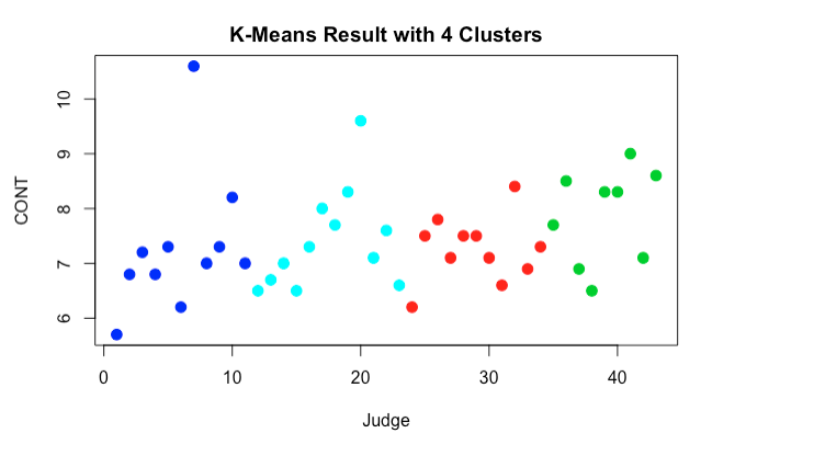
Now, we are plotting the clusters.
# plotting clusters

plot(US_Judge_df , col =(cluster_4$cluster +1) , main="K-Means Result with 4 Clusters", pch=20, cex=2)
What’s next?
The intention of this post was to get familiar with kmeans clustering algorithm concept and its application in R by providing an example. I didn’t analyze the clusters in detail as I didn’t want to make you bored in this post. I’ll write another post to analyze clusters for judge data set.